library(data.table)
library(palmerpenguins)Among the many reasons to use data.table in your code (which includes the more common answers of speed, memory efficiency, etc.) is the syntax. The syntax is
- concise,
- predictable, and
- R-centric.
In this post, I’d like to show how these features are beneficial and useful in working with data regardless of the size of the data. To do this, I’ll use two packages:
and we’ll create a data.table of the penguins data set (and a data.frame version for other examples):
dt <- as.data.table(penguins)
df <- as.data.frame(penguins)
This post assumes some familiarity with data.table syntax but even if you are new to it, there is likely a lot of information that is quite useful for you.
Concise
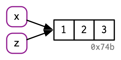
The syntax ultimately is built around the concise dt[i, j, by] framework (built on the core functionality of data frames, see the R-centric section below). This syntax allows you to:
- Subset (“filter”) your data using the
iargument.
# Subset to only Adelie species
dt[species == "Adelie"]
species island bill_length_mm bill_depth_mm flipper_length_mm
<fctr> <fctr> <num> <num> <int>
1: Adelie Torgersen 39.1 18.7 181
2: Adelie Torgersen 39.5 17.4 186
3: Adelie Torgersen 40.3 18.0 195
4: Adelie Torgersen NA NA NA
5: Adelie Torgersen 36.7 19.3 193
---
148: Adelie Dream 36.6 18.4 184
149: Adelie Dream 36.0 17.8 195
150: Adelie Dream 37.8 18.1 193
151: Adelie Dream 36.0 17.1 187
152: Adelie Dream 41.5 18.5 201
body_mass_g sex year
<int> <fctr> <int>
1: 3750 male 2007
2: 3800 female 2007
3: 3250 female 2007
4: NA <NA> 2007
5: 3450 female 2007
---
148: 3475 female 2009
149: 3450 female 2009
150: 3750 male 2009
151: 3700 female 2009
152: 4000 male 2009Other ways to do this include the more redundant base R approach
df[df$species == "Adele"]data frame with 0 columns and 344 rowsand the more verbose approach in the tidyverse.
library(tidyverse)
df %>%
filter(species == "Adele")- Mutate or transform your variables using the
jargument. Note that the use of:=mutates in place so no need for other assignment (e.g.,<-).
# change body_mass_g to pounds
dt[, body_mass_lbs := body_mass_g*0.00220462]
species body_mass_lbs
<fctr> <num>
1: Adelie 8.267325
2: Adelie 8.377556
3: Adelie 7.165015
4: Adelie NA
5: Adelie 7.605939
---
340: Chinstrap 8.818480
341: Chinstrap 7.495708
342: Chinstrap 8.322441
343: Chinstrap 9.038942
344: Chinstrap 8.322441We could also do this in base R a number of ways, all of which are more redundant:
df$body_mass_lbs <- df$body_mass_g*0.00220462
df[, "body_mass_lbs"] <- df[, "body_mass_g"]*0.00220462
df[["body_mass_lbs"]] <- df[["body_mass_g"]]*0.00220462- Do all sorts of data work on groups using the
byargument.
# create a new variable that is the average of the body mass by species
dt[, avg_mass_lbs := mean(body_mass_lbs, na.rm=TRUE), by = sex]
species sex avg_mass_lbs
<fctr> <fctr> <num>
1: Adelie male 10.021507
2: Adelie female 8.514844
3: Adelie female 8.514844
4: Adelie <NA> 8.830728
5: Adelie female 8.514844
---
340: Chinstrap male 10.021507
341: Chinstrap female 8.514844
342: Chinstrap male 10.021507
343: Chinstrap male 10.021507
344: Chinstrap female 8.514844This is more difficult, but possible, in base R to get a summary and add it to the existing data.frame:
tapply(df$body_mass_lbs, df$sex, mean, na.rm=TRUE) # doesn't keep all rows

# does keep all rows but complicated code
df <-
  by(df, INDICES = df$sex,
     FUN = function(x){
       x$avg_mass_lbs <- mean(x$body_mass_lbs)
       return(x)
  })
df <- do.call("rbind", df)
and can definitely be done in the tidyverse.
df <- df %>%
  group_by(sex) %>%
  mutate(avg_mass_lbs = mean(body_mass_lbs, na.rm=TRUE)) %>%
  ungroup()
In each example, you can see a lot of work can be done in a single line of code with minimal redundancy. Although in each situation base R and tidyverse equivalents exist (often with a lot of powerful flexibility in the tidyverse approaches), the concise nature of data.table syntax can make writing and reading the code quicker.
Predictable
The syntax is naturally predictable without being verbose. For instance, whenever you use :=, it’s going to keep the same shape as the current data (“mutate”) while the use of .(var = fun(x)) will summarize to the fewest number of rows appropriate (1 row for non-grouped expressions and x rows for x number of unique groups).
To get an idea of how this predictability manifests in the code, we’ll use an example. Here, we can grab the average bill length by sex. We could do this two ways. The first is mutating in place where the data do not change size or shape. Note, the .() function is shorthand for list().
dt[, avg_bill_length := mean(bill_length_mm, na.rm=TRUE), by = sex]This gives us a new variable in the original data.
       species    sex avg_bill_length
        <fctr> <fctr>           <num>
  1:    Adelie   male        45.85476
  2:    Adelie female        42.09697
  3:    Adelie female        42.09697
  4:    Adelie   <NA>        41.30000
  5:    Adelie female        42.09697
 ---
340: Chinstrap   male        45.85476
341: Chinstrap female        42.09697
342: Chinstrap   male        45.85476
343: Chinstrap   male        45.85476
344: Chinstrap female        42.09697
However, sometimes we just want the data summarized. We can use the syntax below for that (notice no :=).
dt[, .(avg_bill_length = mean(bill_length_mm, na.rm=TRUE)), by = sex] sex avg_bill_length
<fctr> <num>
1: male 45.85476
2: female 42.09697
3: <NA> 41.30000We can always assign this so we can access it later.
avg_bill <- dt[, .(avg_bill_length = mean(bill_length_mm, na.rm=TRUE)), by = sex]One way data.table makes the code predictable is that the data operations happen all within the square brackets without lingering attributes that may produce surprising results. That is, whatever I put in the brackets will be run together and then done. For example, I may have several grouping variables that I use to modify some variables, and only do it for a subset of the data.
dt[species == "Adelie", max_bill := max(bill_length_mm, na.rm=TRUE), by = .(species, sex)]The new variable max_bill is made for the data but is only applicable to the Adelie species and is done by both species as sex. Once this operation is done, the grouping variables are just normal variables again and we still have access to the full data.
       species    sex max_bill
        <fctr> <fctr>    <num>
  1:    Adelie   male     46.0
  2:    Adelie female     42.2
  3:    Adelie female     42.2
  4:    Adelie   <NA>     42.0
  5:    Adelie female     42.2
 ---
340: Chinstrap   male       NA
341: Chinstrap female       NA
342: Chinstrap   male       NA
343: Chinstrap   male       NA
344: Chinstrap female       NA
R-centric
All of the main functionality in data.table is structured around vectors, lists, and (a modified form) of data frames. These core structures in R can be seeing throughout the syntax and design of the package. Even the dt[i, j, by] syntax is designed to mirror (and simplify) data frames. For new users, this can be particularly useful: no additional data structures are needed to work with the data and do both simple and complicated data operations.
Conclusions
In my experience, as one gets more familiar with the syntax of data.table, the more it becomes clear that the syntax (although less verbose than other approaches like the tidyverse), is concise, predictable, and familiar to the basics of the R programming language. Among many reasons to leverage data.table in your workflow, the syntax is one to not overlook.
Cover photo by Christin Hume on Unsplash


Seal of Approval: dtplyr
seal of approval
bridge package
Seal of Approval: nc
seal of approval
extension package

Seal of Approval: tidyfast
seal of approval
bridge package

Announcement: The ‘Seal of Approval’
announcements
grant
community
seal of approval


Announcement: The data.table Ambassadors Travel Grant
announcements
grant
funding opportunity
No matching items